37.2° Blog

1.Model-free RL

Both of the policy iteration and value iteration assume the direct access to the dynamics and rewards of the environment. But, in a lot of real-world problems, MDP model is either unknown or known by too big or too complex to use.

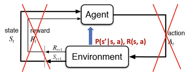
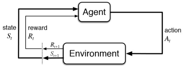
Model-free RL can solve the problems through interaction with the environment

No more direct access to known transition dynamics and reward function

Tarjectories / episodes are collected by the agent's interaction with the environment

Each trajectory / episode contains $\{S_1, A_1, R_1, A_2, R_2,...,S_T, A_T,R_T\}$

2.Model-free prediction

policy evaluation with access to the model

Estimating the expected return of a particular policy if we don't have access to the MDP models:

1. Monte Carlo policy evaluation
2. Temporal Difference (TD) learning

3.Monte Carlo Policy Evaluation

3.1 Overall

蒙特卡洛的方法主要是基于采样的方法，让agent与环境进行交互，得到很多轨迹。每一个轨迹都会得到一个实际的收益。然后直接从实际的收益来估计每个状态的价值

Return : $G_t = R_{t+1} + \gamma R_{t+2} + {\gamma}^2 R_{t+3} + ...$under policy $\pi$

$V_{\pi}(s) = E_{\tau \sim \pi} [G_t| s_t = s]$, thus expectation over trajectories $\tau$generated by following $\pi$

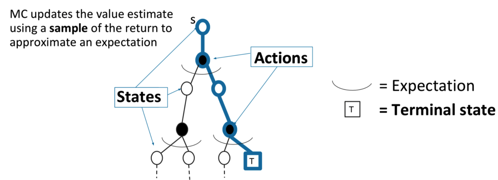
MC simulation : we can simply sample a lot of trajectories, compute the actual returns for all the trajectories, then average them

MC policy evaluation uses empirical mean return instead of expected return

MC does not require MDP dynamics / reward, no bootstrapping, and does not assume state is Markov

Only applied to episodic MDPs(each episode terminates)

3.2 Alg

当要估计某个状态的时候，从这个状态开始通过数数的办法，数这个状态被访问了多少次，从这个状态开始我们总共得到了多少的return，最后再取empirical mean，就会得到每个状态的价值。

To evaluate state V(s)

1. Every time-step $t$ that state $s$ is vistied in an episode
2. Increment counter $N(s) \leftarrow N(s) + 1$
3. Increment total return $S(s) \leftarrow S(s) + G_t$
4. Value is estimated by mean return $v(s) = S(s) / N(s)$

By law of large numbers(大数定律),$v(s) \rightarrow v^{\pi}(s)$ as $N(s) \rightarrow \infty$

3.3 Incremental Mean

写成逐步叠加的办法。

Mean from the average of samples $x_1, x_2, ...$

$$\begin{align} u_t &=\frac{1}{t}\sum_{j=1}^{t}x_j \\ &= \frac{1}{t}(x_t + \sum_{j=1}^{t}x_j) \\ &= \frac{1}{t}(x_t + (t-1)u_{t-1}) \\ &= u_{t-1} + \frac{1}{t}(x_t - v_{t-1}) \end{align}$$

通过采样很多次，就可以平均；然后进行分解，把加和分解成最新的$x_t$的值和最开始到$t-1$的值；然后把上一个时刻的平均值也带入进去，分解成$(t-1)$乘以上一个时刻的平均值；这样就可以把上一个时刻的平均值和这一个时刻的平均值建立一个联系。

通过这种方法，当得到一个新的$x_t$的时候，和上一个平均值进行相减，把这个差值作为一个残差乘以一个learning rate，加到当前的平均值就会更新我们的现在的值。这样就可以把上一时刻的值和这一时刻更新的值建立一个联系。

3.4 Incremental MC Updates

把蒙特卡洛方法也写成Incremental MC更新的方法。

Collect one episode $(S_1, A_1, R_1, ..., S_t)$

For each state $s_t$ with computed return $G_t$

$$N(S_t) \leftarrow N(S_t) + 1 \\ v(S_t) \leftarrow v(S_t) + \frac{1}{N(S_t)}(G_t - v(S_t))$$

Or use a running mean (old episodes are forgotten). Good for non-stationary problems

$$v(S_t) \leftarrow v(S_t) + \alpha (G_t - v(S_t))$$

3.5 Difference between DP and MC for policy evaluation

Dynamic Programming (DP) computes $v_i$ by bootstrapping the rest of the expected return by the value estimate $v_{i-1}$

Iteration on Bellman expectation backup:

$$v_i(s) \leftarrow \sum_{a \in A} \pi(a|s) (R(s,a) + \gamma \sum_{s' \in S}P(s'|s,a)v_{i-1}(s'))$$

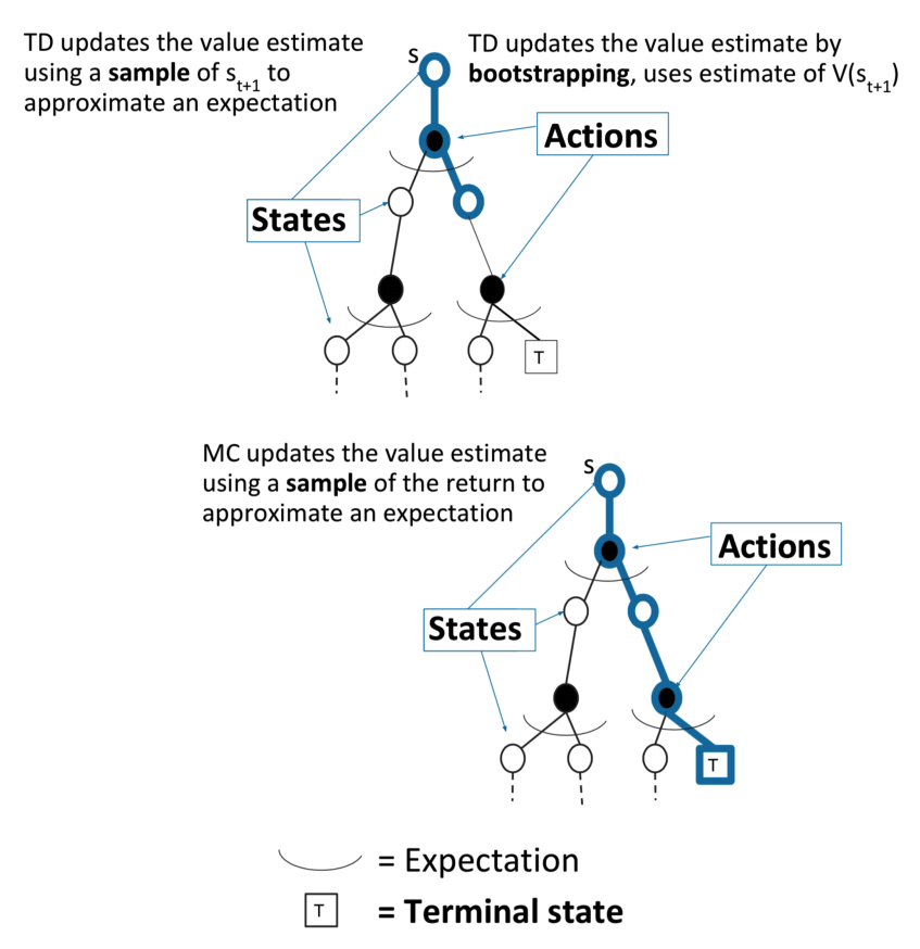
MC updates the empirical mean return with one sampled episode

$$v(S_t) \leftarrow v(S_t) + \alpha(G_{i, t} - v(S_t))$$

3.6 MC相对于DP的优点

1. MC可应用于环境未知（transition function）
2. 对于环境比较复杂的情况，转移概率很难计算，MC基于采样，不需要计算。
3. 计算量的优势：DP要考虑所有的状态转移情况才能更新一步。MC在估计单个状态时与总价值无关。效率更高。

4.Temporal-Difference (TD) Learning

TD是DP和MC折中的一种办法，利用bootstrapping可以从不完整的episode学习。也是基于采样的可用于unknown MDP（transition/rewards）环境中

4.1 Alg : TD(0)

TD(0)指往前看一步。

Objective: learn $v_{\pi}$ online from experience under policy $\pi$

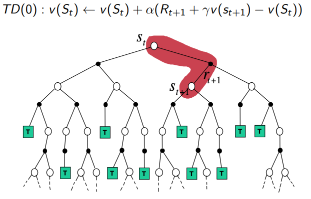
Simplest TD algorithm : TD(0)

Update $v(S_t)$ toward estimated return $R_{t+1} + \gamma v(S_{t+1})$

$$v(S_t) \leftarrow v(S_t) + \alpha(R_{t+1} + \gamma v(S_{t+1} - v(S_t)))$$

$R_{t+1} + \gamma v(S_{t+1})$ is called TD target

${\delta}_t = R_{t+1} + \gamma v(S_(t+1) - v(S_t))$ is called the TD error

Comparison : Incremental Monte-Carlo

Update $v(S_t)$toward actual return $G_t$ given an episode $i$

$$v(S_t) \leftarrow v(S_t) + \alpha(G_{i, t} - v(S_t))$$

4.2 Advantages of TD over MC

1. TD每经过一个timestep都可以更新；MC要等一个episode结束后才能更新。
2. TD可以从不完整的序列学习，MC要用完整的序列才能学习。
3. TD可以用在没有终止状态的环境中，MC不可以。
4. TD利用的MDP的特征（当前状态和之前的状态没有关系），MC并没有利用，它采样并利用了整个轨迹。使得MC在non-Markov环境下更有效。

4.3 n-step TD

n-step TD methods that generalize both one-step TD and MC

We can shift from one to the other smoothly as needed to meet the demands of a particular task.

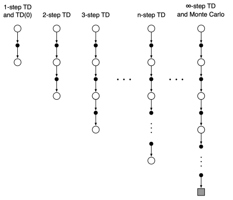
4.4 n-step TD prediction

Consider the following n-step returns for $n = 1,2, ..., \infty$

$$n=1(TD) \space \space \space G^{(1)}_t = R_{t+1} + \gamma v(S_{t+1}) \\ n=2(TD) \space \space \space G^{(2)}_t = R_{t+1} + \gamma R_{t+2} + {\gamma}^2 v(S_{t+1}) \\ ... \\ n=\infty(MC) \space \space \space G^{(\infty)}_t = R_{t+1} + \gamma R_{t+2} + ... + {\gamma}^{T-t-1} R_T$$

Thus the n-step return is defined as

$$G^n_t = R_{t+1} + \gamma R_{t+2} + ... + {\gamma}^{n-1}R_{t+n} + {\gamma}^n v(S_{t+n})$$

n-step TD

$$v(S_t) \leftarrow v(S_t) + \alpha(G^n_t - v(S_t))$$

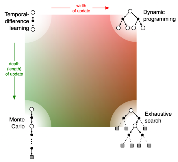
4.5 Bootstrapping and Sampling for DP, MC, and TD

Bootstrapping: update involves an estimate

1. MC does not bootstrap
2. DP bootstraps
3. TD bootstraps

Sampling: update samples an expectation

1. MC samples
2. DP does not sample
3. TD sample

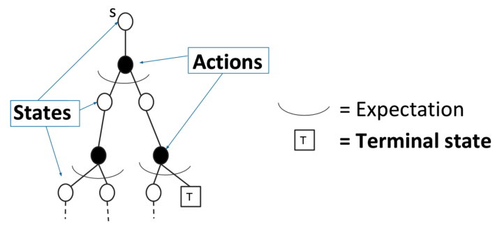
Dynamic Programming Backup

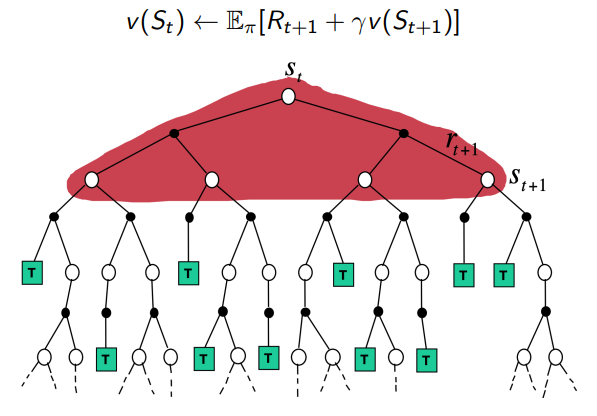
Monte-Carlo Backup

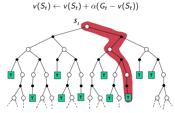
Temporal-Difference Backup

Unified View of Reinforcement Learning

5.Model-free Control for MDP

Model-free Control : Optimize the value function of an unknow MDP

Generalized Policy Iteration (GPI) with MC and TD

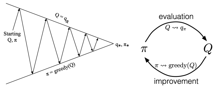
5.1 Policy Iteration

1. Evaluate the policy $\pi$ (computing v given current $\pi$)
2. Improve the policy by acting greedily with respect to $V^{\pi}$

Compute the state-action value of a policy \pi :

$$q^{\pi i}(s, a) = R(s,a) + \gamma \underset{s' \in S}{\sum}{P(s'|s, a)V^{\pi i}(s')}$$

在不知道R和P的情况下，如果获得R(s,a)和P(s'|s,a)并作出决策呢？

5.2 基于MC的广义Policy Iteration

用蒙特卡罗MC的方法取代DP的方法去估计V/Q函数。

用$ε-greedy$方法去改进policy improvement获得$π$。

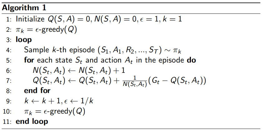
（1）Policy Evalution

原来的policy evalution ：

$$q^{\pi i}(s, a) = R(s,a) + \gamma \underset{s' \in S}{\sum}{P(s'|s, a)V^{\pi i}(s')}$$

现在MC的 Policy evalution

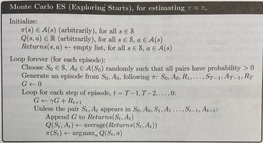
（2）Policy Improvement

考虑 exploration 和 exploitation 的 tradeoff 的问题。

Trade-off between exploration and exploitation (we will talk about this in later lecture)

$ε-Greedy$ Exploration : Ensuring continual exploration

1. All actions are tried with non-zero probability
2. With probability $1 - ε$ choose the greedy action
3. With probability $ε$ choose an action at random

$${\pi}(a|s) = \left \{ \begin{aligned} \epsilon / |A| + 1 - \epsilon, &\space if \space a^* = argmax_{a \in A} \space {Q(s,a)} \\ \epsilon / |A|, &\space otherwise \\ \end{aligned} \right.$$

5.3 基于TD的广义Policy Iteration

（1）MC vs TD

TD相比MC的优势：方差小、在线的、处理不完整的序列

用TD的方法可以取代DP/MC的方法去估计V函数。同样用$ε-greedy$方法去改进policy improvement获得$π$。那如何使用TD的方法获得$Q(s,a)$呢？

（2）On-Policy 和 Off-Policy 的对比

On-Policy：学习过程中只利用我们现在正在学的这个策略$π$，采集轨迹数据和优化策略始终都是用这个策略$π$。

Off-Policy：保留两个策略，一个是我们要优化的目标策略 target $π$ ，另一个是探索的策略 action $μ$ 。探索的策略$μ$就可以更激进，并通过 $μ$ 来采集数据，采到的数据给 $π$ 去学习。

Off-Policy benefits:

1. Learn about optimal policy while following exploratory policy
2. Learn from observing humans or other agents
3. Re-use experience generated from old policies $π_1, π_2, ..., π_{t-1}$

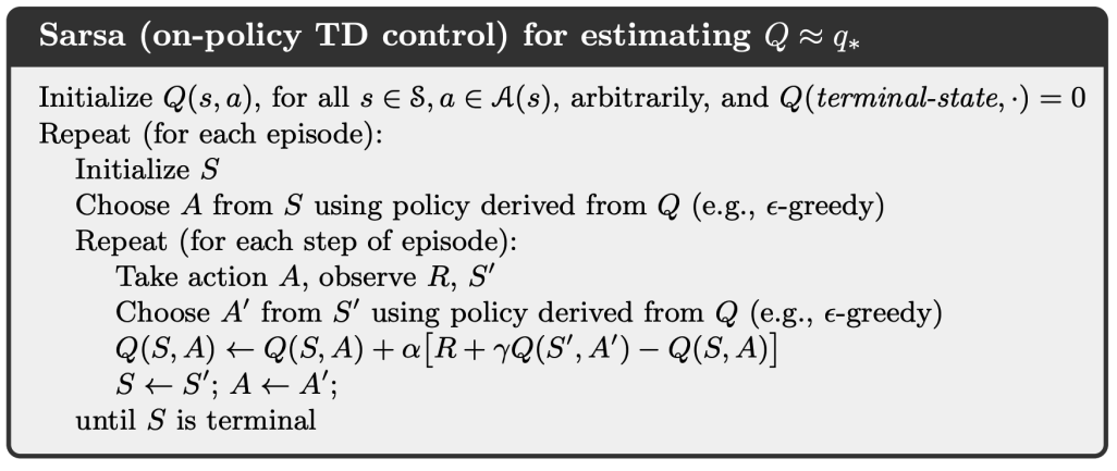
（3）On-Policy TD control：Sarsa

（S A R S A 进行循环的意思）

An episode consists of an alternating sequence of states and state-action pairs:

$ε-greedy$ policy for one step, then bootstrap the action value function:

$$Q(S_t, A_t) \leftarrow Q(S_t, A_t) + \alpha[R_{t+1} + \gamma Q(S_{t+1}, A_{t+1}) - Q(S_t, A_t)]$$

The update is done after every transition from a nonterminal state $S_t$

TD target $\delta_t = R_{t+1} + \gamma Q(S_{t+1}, A_{t+1})$

Sarsa algorithm

（4）n-step Sarsa

Consider the following n-step returns for $n = 1,2, ..., \infty$

$$n=1(Sarsa) \space \space \space q^{(1)}_t = R_{t+1} + \gamma Q(S_{t+1}, A{t+1}) \\ n=2(TD) \space \space \space q^{(2)}_t = R_{t+1} + \gamma R_{t+2} + {\gamma}^2 Q(S_{t+2}, A{t+2}) \\ ... \\ n=\infty(MC) \space \space \space q^{(\infty)}_t = R_{t+1} + \gamma R_{t+2} + ... + {\gamma}^{T-t-1} R_T$$

Thus the n-step return is defined as

$$q^n_t = R_{t+1} + \gamma R_{t+2} + ... + {\gamma}^{n-1}R_{t+n} + {\gamma}^n Q(S_{t+n}, A{t+n})$$

n-step TD

$$Q(S_t, A_t) \leftarrow Q(S_t, A_t) + \alpha(q^n_t - Q(S_t, A_t))$$

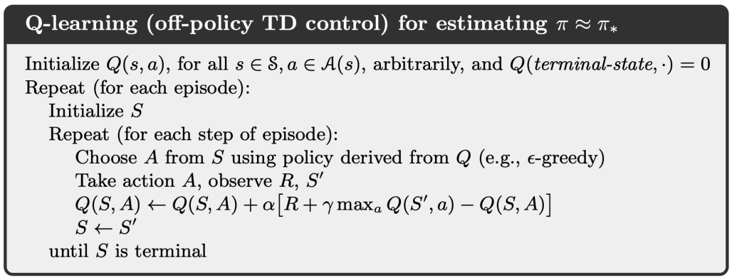
（5）Off-Policy TD control：Q-learning

We allow both behavior and target policies to improve

The target policy $π$ is greedy on $Q(s, a)$

$$\pi(S_{t+1}) = \underset{a'}{arg \space max \space } Q(S_{t+1}, a')$$

The behavior policy $µ$ could be totally random, but we let it improve。

following $ε-greedy$ on $Q(s, a)$

Thus Q-learning target：

$$R_{t+1} + \gamma Q(S_{t+1}, A') \\ = R_{t+1} + \gamma Q(S_{t+1}, arg \space max \space Q(S_{t+1}, a')) \\ = R_{t+1} + \gamma \underset{a'}{max \space } Q(S_{t+1}, a')$$

Thus the Q-Learning update

$$Q(S_t, A_t) \leftarrow Q(S_t, A_t) + \alpha[R_{t+1} + \gamma \underset{a'}{max \space }Q(S_{t+1}, a) - Q(S-t, A_t]$$

Q-learning algorithm

（6）Sarsa和Q-learning的区别

1. Sarsa是只利用一个策略π，而Q-Learning有两个策略π和μ

Sarsa : On-Policy TD control

Choose action $A_t$ from $S_t$ using policy derived from $Q$ with $ε-greedy$ Take action $A_t$, observe $R_{t+1}$ and $S_{t+1}$ Choose action $A_{t+1}$ from $S_{t+1}$using policy derived from $Q$ with$ε-greedy$ $Q(S_t, A_t) \leftarrow Q(S_t, A_t) + \alpha[R_{t+1} + \gamma Q(S_{t+1}, A_{t+1}) - Q(S_t, A_t)]$

Q-Learning: Off-Policy TD control

Choose action $A_t$ from $S_t$ using policy derived from $Q$ with $ε-greedy$ Take action $A_t$, observe $R_{t+1}$ and $S_{t+1}$ Then ‘imagine’$A_{t+1}$as arg max $Q(S_{t+1}, a')$ in the update target $Q(S_t, A_t) \leftarrow Q(S_t, A_t) + \alpha[R_{t+1} + \gamma \underset{a'}{max \space }Q(S_{t+1}, a) - Q(S-t, A_t]$

2. backup diagram过程不同

Backup diagram for Sarsa and Q-learning

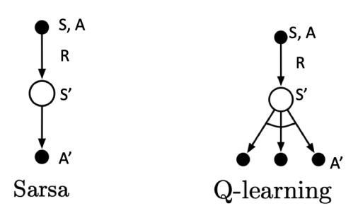
In Sarsa, $A$ and $A'$ are sampled from the same policy so it is on-policy

In Q Learning, $A$and $A'$ are from different policies, with $A$ being more exploratory and $A'$ determined directly by the max operator

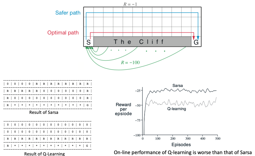
3.Sarsa更保守，Q-Learning更激进冒险

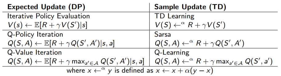
5.4 DP vs TD